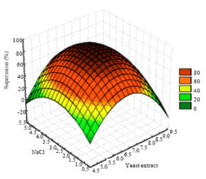
Though, the technique of ‘Statistical Experimental Design’ has been around from 1930’s; it was accepted by the industry, largely due to simplification efforts of Dr. Taguchi. The rapid acceptance of Dr. Taguchi methods of ‘Robust Design’ prompted a debate (which is still going on) “Classical DOE vs. Taguchi Methods of Robust Design – Which is better?”
Adding to the complexity is the new technique of experimental – RSM. Though, the Taguchi Methods are the most efficient way for optimisation; at times, the engineer may require a method of optimisation which accounts for the interaction effects, if any. Further, in the era of wafer-thin margins/ contribution; the design engineer may seek to fin-tune the settings of the control-factors/ design parameters to get that extra competitive advantage. It is under these demanding situations, where advanced tools like RSM could play a significant role.
The difference between Classical Taguchi Methods, DOE, and RSM is elaborated in the following table.
| Taguchi Methods | Classical DOE | RSM | |
| Objective | · To estimate an optimum setting for a product/process, in terms of its control factors and their design levels.
e.g., if y= f(A1/2/3, B1/2/3, C1/2/3), identify combination of A,B & C at their levels 1/2/3 for an optimum y · The objective is always to maximise the S/N ratio of the response. |
· To develop a linear (1st order) function to describe a product/process performance and use the equation to set the product/process at its optimum setting.
e.g., if y=f(x1,x2,x3), estimate the equation: y=a0 +a1x1 +a2x2 +a3x3 +a12x1x2 +a13x1x3 +a23x2x3 +a123x1x2x3 · Based on the objective of design, y is set at minima/maxima or its nominal value.
|
· To develop a quadratic (2nd order) function to describe a product/process performance and use the equation to set the product/process at its optimum setting.
e.g., if y=f(x1,x2,x3), estimate the equation: y=a0 +a11x12 +a22x22 +a33x32 +a1x1 +a2x2 +a3x3 +a12x1x2 +a13x1x3 +a23x2x3 +a123x1x2x3 · Based on the objective of design, y is set at minima/maxima or its nominal value.
|
| Experimental Plans |
|
|
|
| Factors | Factors could be both continuous or discrete | Factors could be continuous or discrete | Factors must be continuous variables! |
| Analysis | Using the ‘Average Effect Plots’ the factors are set at their respective levels where the average-effect of the S/N ratio is maximum. | Using multiple linear regression, the mathematical model is developed. Using the equation the optimum setting for the product/process is arrived at. | In case of Central Composite Designs (CCDs):
Box & Behnken Designs: These designs are deployed when the product/process performance is known to follow a quadratic equation. The quadratic equation is directly estimated using the regression tool |
Summing up, when conducting experiments is an expensive affair, Taguchi Methods present a cost effective alternative. They are easy to plan and the analysis involved requires simple computation. If one is interested in studying interactions, then the Classical DOE presents itself as an appropriate tool. If the engineer is not sure whether the product/process performance follows a linear equation or quadratic equation, he/she could use the CCD. If the engineer is confident that the product/process performance follows a quadratic equation, he/she could use the ‘Box & Behnken Design’ plan.
Recommended path
- Start the development work with many factors (short-listed after brain-storming)
- Use Taguchi Methods as ‘Screening Experiments’ to reduce the list of potential factors and reduce the experimental effort.
- Use Classical DOE (Full Factorial) to verify whether the product/process performance follow a linear function.
- If Yes, deploy the method of steepest ascent/descent
- If analysis indicate a presence of a curvature, conduct additional runs as per RSM


